\section{Black-Scholes-Merton Model}\label{sec:BSM}
Consider a financial asset whose spot price is measured by a stochastic process $S_t$. It has been shown that (see \cite{Cont2001}), in general, it is not the differences $S_{t+1}-S_t$ that are independent but the rates of return
\begin{equation}\label{eq:BSMM.5} \frac{S_{t+1}-S_t}{S_t}\approx\frac{dS_t}{S_t} , \quad\text{ for }t\in\left(0,T\right). \end{equation}If we assume that $\displaystyle\frac{dS_{t}}{S_t}$ is a BM with drift then
\begin{equation}\label{eq:BSMM.10} \frac{dS_t}{S_t} = \mu dt +\sigma dZ_t\Leftrightarrow dS_t= \mu S_t dt +\sigma S_t dZ_t \end{equation}for some constants $\mu$ and $\sigma$, with the standard BM $Z_t$. To proceed, we need to refer to Itô's Lemma.
\begin{lemma}\label{lemma:Ito} If $X_t$ is a BM with drift, i.e., $dX_{t} = \mu dt +\sigma dZ_t$ and $f(t,x)$ a twice differentiable function then $$ df(t,X_t) = \left(\frac{\partial f}{\partial t}+\frac{1}{2}\sigma^2\frac{\partial^2 f}{\partial X_t^2}\right)dt+ \frac{\partial f}{\partial X_t}dX_t. $$ \end{lemma}Using the MacLaurin series, we know that $\log(1+x)\approx x$. From this fact, we have that the rate of return above is given approximately as $\log\left(S_{t+1}\right)-\log\left(S_{t}\right)$ So it is natural that, instead to look to the time series of $S_t$, we are more interested in the $\log\left(S_{t}\right)$ series. Applying Lemma \ref{lemma:Ito} to equation (\ref{eq:BSMM.10}), we found that the process $d\log\left(S_{t}\right)$ given in (\ref{eq:BSMM.10}) is equivalent to
\begin{equation}\label{eq:BSMM.20} d\log S_t = \left(\mu -\frac{1}{2}\sigma^2\right)dt + \sigma dZ_t. \end{equation}Using (\ref{eq:BSMM.5}), this shows that the solution of equation (\ref{eq:BSMM.20}), for $t\in(0,T)$, is
\begin{equation}\label{eq:BSMM.30} S_t = S_0\exp\left(\left(\mu -\frac{1}{2}\sigma^2\right)t + \sigma Z_t\right). \end{equation}Indirectly we have proved that $S_t=S_0\exp \left(\left(\mu -\frac{1}{2}\sigma^2\right)t + \sigma Z_t\right)$ is the solution of equation (\ref{eq:BSMM.20}). Because of this we say that $S_t$ is a Geometric Brownian Motion. We also know that $S_t$ has a lognormal distribution and this is the starting point for the deduction of the Black-Scholes-Merton Formula.
Again, for some partition of the interval $0<t_1<\dots<t_N=T$ we can use expression (\ref{eq:BSMM.30}) to find the discretization of the process $S_t$
\begin{equation}\label{eq:BSMM.40} S_{t_{i+1}} = S_{t_{i}}\exp\left(\left(\mu-\frac{\sigma^2}{2}\right)\Delta+\sigma\sqrt{\Delta}G_{i+1}^S\right). \end{equation}This is the formula that we are going to use for the simulation of the asset price dynamics. Regard that in this quite unrealistic case we know the final distribution of the process. Because of this there is no need to make simulations to compute the expected value of the asset price in future time. However, because we focus essentially in making simulations, this example may be quite rewarding for the general comprehension of the method.
using Plots
# The computation of an individual orbit of the asset price

nsteps = 500 # number of subintervals in (0,T)
initial_t = 0
# recall that our time is always fractions of years
final_t = 30/365
delta = (final_t - initial_t)/nsteps
stdsigma = sqrt(delta)

tempo = linspace(initial_t , final_t , nsteps)

# we need to use the correct value of the interest rate
# from the yearly interest rate, we have to actualize it to the fraction of the year used
# r_TTM = r * TTM, where TTM units is days/365
# because we split TTM in nsteps intervals, the effective interest rate is r * delta.
driftfunc(t) = 0.06 * delta
volfunc(t) = 0.25

drift = map(driftfunc,tempo)
vol = map(volfunc,tempo)

spot = 100.0


gaussval = randn(nsteps)

expoente = (drift - 0.5 * delta * vol.^2) + sqrt(delta) * vol .* gaussval
asset_price = spot * cumprod(map(exp,expoente))

plot(tempo,asset_price,legend = false)
We can use the ideas in the previous code to automate the path simulation of asset price.
function simulatepath(initial , final , nsteps , driftval , volval, spot)
    delta = (final_t - initial_t)/nsteps
    stdsigma = sqrt(delta)

    tempo = linspace(initial_t , final_t , nsteps)
    driftfunc(t) = driftval * delta
    volfunc(t) = volval

    drift = map(driftfunc,tempo)
    vol = map(volfunc,tempo)

    gaussval = randn(nsteps)

    expoente = (drift - 0.5 * delta * vol.^2) + sqrt(delta) * vol .* gaussval

    return spot * cumprod(map(exp,expoente))
end
initial_t = 0
final_t = 10/365
nsteps = 500
driftval = 0.01
volval = 0.25
spot = 100

tempo = linspace(initial_t,final_t,nsteps)
asset_path = simulatepath(initial_t , final_t , nsteps , driftval , volval , spot)

plot(tempo,asset_path, legend = false)
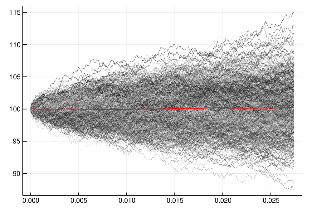
Now, we can simulate a lot of paths and compute the average path.
initial_t = 0
final_t = 10/365
nsteps = 500
driftval = 0.01
volval = 0.25
spot = 100

npaths = 500

tempo = linspace(initial_t,final_t,nsteps)
asset_path = simulatepath(initial_t , final_t , nsteps , driftval , volval , spot)
# the mean path is equal to the first path when there is only one.
media = asset_path

plot(tempo,asset_path,legend = false, palette=:grays,lw = 0.2);

for i in 1:npaths
    asset_path = simulatepath(initial_t , final_t , nsteps , driftval , volval , spot)
    plot!(tempo,asset_path,legend = false,palette=:grays,lw = 0.2)

    # before increment i update mean_path
    media = (1-1/(i+1)) * media + (1/(i+1)) * asset_path
end

plot!(tempo,media,legend = false,color=:red,lw = 1.2);
savefig("teste.pdf")
# you can convert this to a web format via gs using
# gs -sDEVICE=pngalpha -o simulation.png -r200 teste.pdf
HTML("""
    <img src="simulation.png" />
    """)
It is easy at this moment to compute the value of an European Call or Put Option under the BSM framework. Given a financial asset whose value is measured by a Geometric Brownian Motion $S_t$, for a time to maturity (TTM) T, a spot price S and a interest rate r, then
\begin{equation}\label{eq:BSMM.50} C=\exp(-rT)\,\mathbb{E}\left((S_T-K)^+\right)\text{ and } P=\exp(-rT)\,\mathbb{E}\left((K-S_T)^+\right). \end{equation}To compute the value of $S_T$ we will produce simulations of the path of the asset price and keep the last value. We then increment the average in the usual way. We start by defining the maxplus function.
function maxplus(x)
    out = 0
    if x > 0
        out = x
    end
    return out
end
initial_t = 0
final_t = 30/365
nsteps = 250
driftval = 0.01
volval = 0.25
spot = 9.51
strike = 9.0

npaths = 200000

# tempo = linspace(initial_t,final_t,nsteps)
asset_path = simulatepath(initial_t , final_t , nsteps , driftval , volval , spot)

# The call and put values initialization
callvalue = maxplus(asset_path[nsteps]-strike)
putvalue = maxplus(strike - asset_path[nsteps])

for i in 1:npaths
    asset_path = simulatepath(initial_t , final_t , nsteps , driftval , volval , spot)
    # before increment i update mean_path
    callvalue = (1-1/(i+1)) * callvalue + (1/(i+1)) * maxplus(asset_path[nsteps]-strike)
    putvalue = (1-1/(i+1)) * putvalue + (1/(i+1)) * maxplus(strike - asset_path[nsteps])
end

callvalue = exp(-driftval * (final_t - initial_t)) * callvalue
putvalue = exp(-driftval * (final_t - initial_t)) * putvalue

println("The price of European Call Option is $(callvalue)")
println("The price of European Put Option is $(putvalue)")
We reinforce the idea that the BSM framework is useful for us because it is a very good learning playground. In this framework running simulations is not the best method to compute the price of European Options. The reason for this is due to the existence of the famous Black-Scholes-Merton formula. However, and because of the existence of this formula, we have a benchmark to which we can compare the results of our simulations. This, when we are willing to learn how to do things, it is priceless.
References
(Cont, 2001) Cont R., ``Empirical properties of asset returns: stylized facts and statistical issues'', Quantitative Finance, vol. 1, number 2, pp. 223-236, 2001.